Internship research · StratiFi Solutions
Dynamic Equity–Bond Allocation
Volatility signals, rolling evaluation, and model interpretation
Diversification reduced average equity correlation, but left substantial crisis drawdowns. I investigated whether volatility states could guide equity–bond exposure, then examined how the allocation policy behaved outside its fitting windows.
The research uses 503 S&P 500 equity records over January 2015–September 2024. PCA transforms 22-, 44-, and 132-day volatility measures into level, slope, and curvature signals. Linear and tree-based policies map those signals to allocation weights. The workflow progresses from in-sample optimization to rolling fits, SHAP interpretation, and an extension using volume volatility.
Rolling allocation behavior
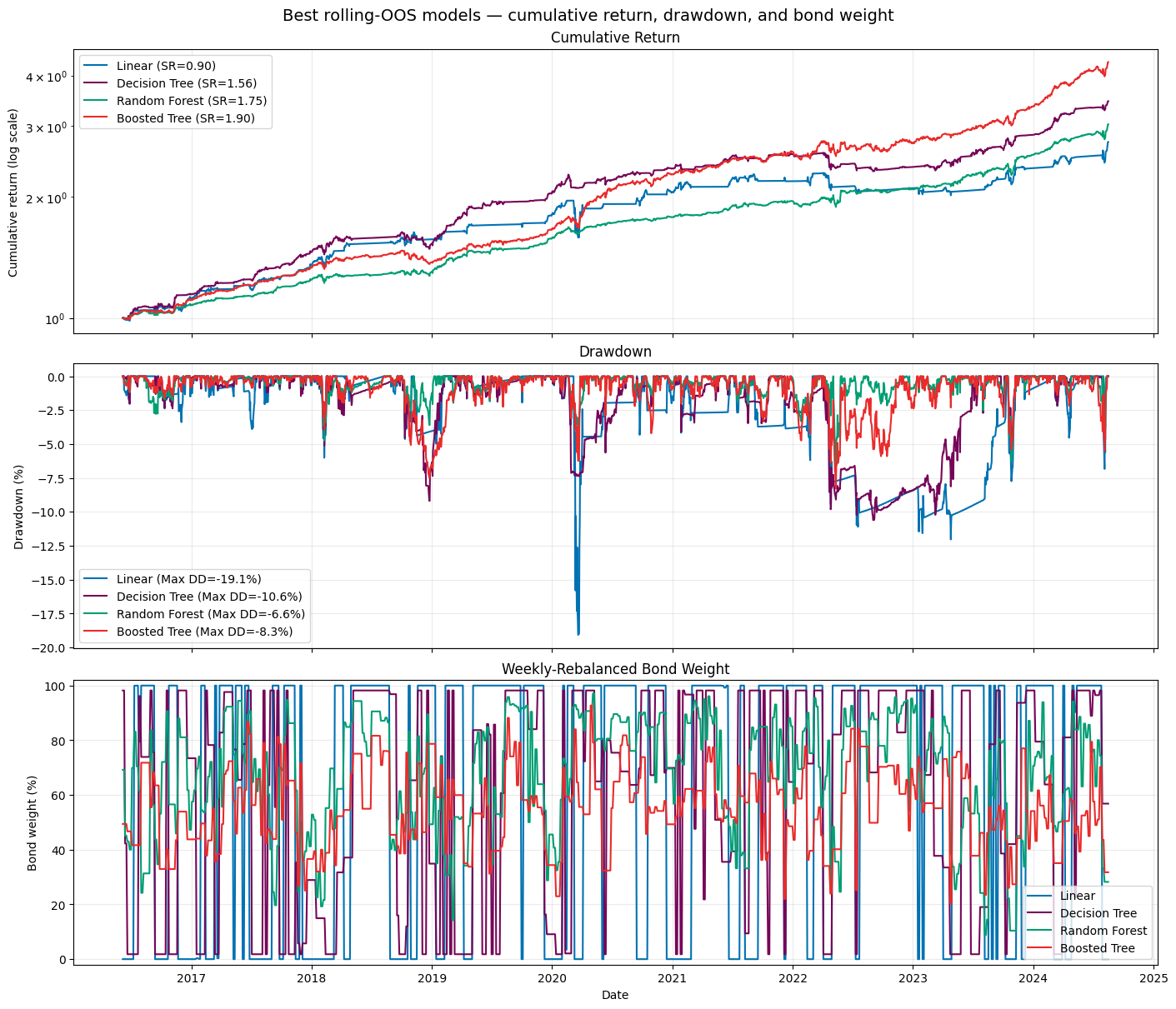
Each window fits the scaler, PCA, and policy on 48 weeks, predicts the following four weeks, and advances four weeks. The presentation reports 107 non-overlapping test blocks and 2,140 daily observations. XGBoost has the highest stitched Sharpe among the four policies shown, although random forest has the smaller maximum drawdown.
Adding trading-activity information
The six-component XGBoost model adds PCA features from volume volatility. Reported rolling-evaluation Sharpe increases from 1.8996 to 1.9441, while maximum drawdown improves from −8.28% to −8.05%. The presentation’s decomposition attributes 0.0052 of the Sharpe increase to additive volume effects and 0.0393 to cross-group interactions.
| Specification | Evaluation | Sharpe | Ann. excess return | Max. drawdown |
|---|---|---|---|---|
| 3-PC XGBoost | In-sample | 2.6030 | 11.17% | -2.79% |
| 3-PC XGBoost | Rolling evaluation | 1.8996 | 15.45% | -8.28% |
| 6-PC XGBoost | Rolling evaluation | 1.9441 | 16.47% | -8.05% |
Source: slides 9–12. “Annualized excess return” follows the presentation’s label; it should not be read as outperformance over SPY. Figures are not net of transaction costs.
SHAP rankings also change between the in-sample and rolling analyses: the volatility level dominates in-sample, while the slope becomes more important in rolling evaluation. This motivates testing state-dependent interactions, while recognizing that feature attribution is descriptive rather than causal.
Data construction, limitations & next steps
The source panel contains daily prices, market capitalization, and volume. Returns use a market-cap-based proxy to avoid raw split jumps; missing inputs are forward-filled and imputed-date returns are set to zero. SPY is the broad-market benchmark, and FRED DGS2 is a yield-based bond proxy rather than a realistic bond total-return series.
The presentation explicitly identifies upstream look-ahead from full-sample stock selection and weight optimization, along with selection bias from tuning on rolling-test performance. Consequently, the reported Sharpe ratios do not establish fully independent end-to-end out-of-sample performance.
Next steps are to re-select stocks and fit weights within training windows, use nested tuning with an untouched holdout, and evaluate actual bond total returns with trading costs and turnover penalties. Broader market-state signals and allocation stability constraints remain directions for further work.
Source: StratiFi End of Internship Presentation, August 9, 2026, slides 3–14. The chart is extracted unchanged from the supplied presentation.